Long Beach City College Retention Analysis
Posted on Tue 20 December 2016 in Projects
Background information
With the support of the Institutional Research Department at Long Beach City College, I was given 10 years of college wide student data to provide them with any insights. For the purpose of privacy, the data will not be displayed in this notebook. However, I can provide desciptions and the variables that are being used along with results from the analysis. The data was given to me in three tables, enrollment, miscellaneous, and awards.
The topic that interests me about education data is determining patterns to improve the retention and persistance rates. Retention and persistance is one of, if not the most, important topics in higher education.
After doing some research and speaking with a few people in education, many institutions use the probation rule to flag students as "at risk"; the student is on probation if he/she has a gpa of 2.0 or less. Once a student is on probation, the college reaches out to the student to offer early intervention and provide the students with additional resources to improve their academics. The detailed policy for Long Beach City College can be found from this link : http://www.lbcc.edu/Admissions/documents/Probation%20and%20Dismissal%20FAQS.pdf
The goal of my analysis is use machine learning models to further improve the "at risk" flagging system that many institutions use today. If schools can have a better basis and understanding of which students are more likely to be at risk, they can effectively allocate resources and help many more students persist.
### Code to configure RISE Reveal.js presentation from notebook cells
from IPython.html.services.config import ConfigManager
from IPython.utils.path import locate_profile
cm = ConfigManager(profile_dir=locate_profile(get_ipython().profile))
cm.update('livereveal', {
              'theme':'sansserif',
              'slideNumber': True,
              'width': 1300,
              'height': 900,
              'scroll': True,
})
Data
Enrollment Table
| Variable | Description |
|---|---|
| studentid | Student id number for identification |
| ay | Academic Year in which course was taken |
| term | Term in which course was taken |
| subject | subject code of course |
| course | course code |
| section | section number |
| unitsattempted | total units course is worth |
| grade | grade earned in course |
| gender | gender |
| eth | ethnicity |
| firstterm | first term the student enrolled at LBCC |
| samcode | Course vocational status |
| wdegapp | Whether or not a course is degree applicable (basic skills courses do not count toward an AA/AS degree) |
| transstat | Transfer Status of the course |
| location | Campus where course was taught or online course |
Miscellaneous Table
| Variable | Description |
|---|---|
| studentid | Student id number for identification |
| wveteran | 1 if the student is a Veteran, 0 if not. |
| wbog | 1 if the student has ever received the Board of Governors Fee Waiver, 0 if not. |
| wpell | 1 if the student has ever received a Pell Grant, 0 if not. |
| edgoaldes | Educational Goal as stated on their application to LBCC |
| highestedlevel | The highest education level they attained upon entering LBCC |
| firstgeneration | 1 if the both parents did not attend any college, 0 if any parent attended college, -99 if data is unavailable |
| readplacement | Highest Read placement on our assessment exams |
| mathplacement | Highest Math placement on our assessment exams |
| englplacement | Highest English placement on our assessment exams |
| plandes | student major |
| wfoster | 1 if the student was in the foster youth system, 0 if not. |
Awards Table
| Variable Name | Description |
|---|---|
| studentid | Student id number for identification |
| Major | Major in which student earned award |
| Award | Type Certificate or AA/AS |
| Award Term | Term in which Award was earned |
from IPython.display import Image

import pandas as pd
import numpy as np
from copy import copy
import pydotplus

import pandas as pd
import numpy as np
from sqlalchemy import create_engine
import sqlite3
import psycopg2

from sklearn.model_selection import train_test_split
from sklearn.model_selection import GridSearchCV

from sklearn.preprocessing import normalize
from sklearn.metrics import precision_recall_fscore_support


from sklearn.linear_model import LogisticRegression
from sklearn.neighbors import KNeighborsClassifier
from sklearn.svm import SVC
from sklearn.neural_network import MLPClassifier

from sklearn.ensemble import GradientBoostingClassifier
from sklearn.ensemble import VotingClassifier
from sklearn.tree import DecisionTreeClassifier
from sklearn.tree import export_graphviz
# from sklearn.ensemble import RandomForestClassifier
# from sklearn.naive_bayes import GaussianNB

from sklearn.metrics import confusion_matrix
from sklearn.metrics import auc, roc_curve
from sklearn.metrics import precision_recall_curve
from sklearn.metrics import log_loss
from sklearn.metrics import f1_score

from sklearn.cluster import KMeans
from sklearn.cluster import SpectralClustering
from sklearn.decomposition import PCA

import xgboost as xgb

from imblearn.over_sampling import SMOTE
from imblearn.under_sampling import CondensedNearestNeighbour
from imblearn.under_sampling import RandomUnderSampler

import category_encoders as ce

import seaborn as sns
import matplotlib.pyplot as plt
import matplotlib.image as mpimg
from matplotlib import gridspec
%matplotlib inline
award = pd.read_csv('awards.csv')
enrollments = pd.read_csv('enrollments.csv')
misc = pd.read_csv('mis_student_data.csv')
Research Problem:
- Using students' first semester of data, identify if students will return for a 3rd semester
- The goal is to intervene early to provide students with resources, to increase retention
Data
The enrollment table has 2,293,687 rows and 16 columns. The awards table has 30,429 rows and 4 columns. The miscellaneous table has 198,981 rows and 12 columns.
The inital data needed to be cleaned. The data was exported using SPSS so many of the data types did not agree, even within a column, i.e. half of the wdegapp (1 if the class is applicable to degree 0 otherwise) values 1 and 0 were integers, and the other were strings. Thus, the first thing I did was each column to its appropriate data types.
# award.head()
# misc.head(4)
# enrollment.iloc[190000:190005]
pd.set_option('display.max_columns', 300)
enrollments.head()

''' Enrollment dataframe seems to contain empty columns.
These columns are likely to be for the list of courses.
We will search for when the student data begins **
'''

enrollments[183760:].head()

#The data seems to start on the 183766th row

enrollment = enrollments[183766:].reset_index().drop('index',axis = 1)

#Let's make sure that the number of student data given is consistent across the tables

''' There seems to be a problem and mismatch in the amount of information given on students between
the misc and enrollment dataset. One possibility is the dtype of the columns.
We will convert the column types and see if that helps.
'''

misc['studentid'] = misc['studentid'].astype(str)
enrollment['studentid'] = enrollment['studentid'].astype(str)

''' That seem to have fixed the issue.
However, it seems like the data has different dtypes within the column so we will convert each
column one by one to the correct dtype to work with.
'''

dtypes_enrollment = ['int','int','str','str','int','float','str','str','str','str','int','str','str',
                     'float','str','str']

''' There is an issue with the wdegapp column as there are different values and also missing values.
We will fix that by imputing the empty values with a zero.
'''

enrollment.ix[enrollment['wdegapp'] == ' ', 'wdegapp'] = 0

col_name = enrollment.columns.values
for i in range(len(dtypes_enrollment)):
    enrollment[col_name[i]] = enrollment[col_name[i]].astype(dtypes_enrollment[i])

''' Conversion of dtypes for enrollment table seems successful.
We will now do the same for the award and misc table.
'''

dtype_award = ['str','str','int','str']


award['awardterm'].unique()

'''There seems to be the same issue with the award table for the awardterm column.
We will fill the empty values with a -99.
'''

len(award[award['awardterm'] == ' '])

award.ix[award['awardterm'] == ' ', 'awardterm'] = -99.0

col_name_award = award.columns.values
for i in range(len(col_name_award)):
    award[col_name_award[i]] = award[col_name_award[i]].astype(dtype_award[i])

dtype_misc = ['str','float','float','float','str','str','float','str','str','str','str','float']

col_name_misc = misc.columns.values
for i in range(len(col_name_misc)):
    misc[col_name_misc[i]] = misc[col_name_misc[i]].astype(dtype_misc[i])

''' All tables seem to be clean now. We will now join the three tables on the student id column
and then export the dataframe into a SQL database
'''
I started to engineer a few features from here.
First, using the grade each student received in each course, I created a new column that holds the value of the grade, i.e. A = 4.0, B = 3.0, etc.
In attempt to capture the difficulty of each course offered by the college, I looked at the distribution of each course over the span of 10 years and assigned a course weight to each course. For example, if a majority of the students over 10 years earned A's in a course, then the course weight given to that course is a 1. Conversely, a course weight of 5 is given to a course that has a majority of students earning F's.
# Create feature for class difficulty based on prior performance (probability)

course_dist = pd.crosstab(enrollment['grade'], enrollment['course']).iloc[1:]
# course_dist = course_dist.drop('UG', axis = 0)

#Define course weight

courses = course_dist.columns
np.argmax(course_dist[courses[9]])


# index:  A   - 0     Weight: 1
#         B   - 2     Weight: 2
#         C/P - 3/10  Weight: 3
#         D   - 4     Weight: 4
#         Rest/F -    Weight 5

course_weight = np.zeros(len(courses))
count = 0
for course in courses:
    if (np.argmax(course_dist[course]) == 'A') | (np.argmax(course_dist[course]) == 'UG') :
        course_weight[count] = 1
    elif np.argmax(course_dist[course]) == 'B':
        course_weight[count] = 2
    elif (np.argmax(course_dist[course]) == 'C') | (np.argmax(course_dist[course]) == 'P') :
        course_weight[count] = 3
    elif np.argmax(course_dist[course]) == 'D':
        course_weight[count] = 4
    else:
        course_weight[count] = 5
    count += 1

enrollment = enrollment.merge(pd.DataFrame({'course_weight':course_weight, 'course': courses}),
                              on = 'course', how = 'left')
misc.head()
df = enrollment.merge(misc, on = 'studentid', how = 'left')
df = df.merge((award.drop_duplicates('studentid')), on = 'studentid', how = 'left')
df['grade_value'] = np.zeros(len(df))

# Create grade value column to calculate gpa

df.ix[df['grade'] == 'P', 'grade_value'] = 2.0
df.ix[df['grade'] == 'A', 'grade_value'] = 4.0
df.ix[df['grade'] == 'B', 'grade_value'] = 3.0
df.ix[df['grade'] == 'C', 'grade_value'] = 2.0
df.ix[df['grade'] == 'D', 'grade_value'] = 1.0

# df.to_csv('student_df.csv')

# engine = create_engine('postgresql://truong:****@localhost:5432/lbcc_truong')
# df.to_sql('studentdata',engine, chunksize = 100000)
Next, to slice the data to attain only 1st semester of data on each student, it was best to port this cleaned dataset from a csv file to a PostgresSQL database for efficiency and speed.
pd.set_option('display.max_columns',200)

con = psycopg2.connect(dbname = 'lbcc_truong', host = 'localhost', user = 'postgres', password = '**')
cur = con.cursor()
SQL Query
- Find students who have taken at least 3 semesters of courses
- These students will be given label 1 and the students that are not on this list will be given label 0
- Construct dataset of students' first semester data
- Features that were engineered from enrollments table:
- GPA
- Most recent GPA (previous semester)
- Average GPA
- Total class weight
- Maximum number of courses taken (of all semesters)
- Minimum number of courses taken (of all semesters)
- Total number of degree applicable courses taken
- Total number of transferrable courses taken (UC + CSU)
- Total units attempted
- Total online courses taken
- Total classroom courses taken
student_list = pd.read_sql_query(
'''
SELECT studentid
FROM(
    SELECT DISTINCT ON (studentid)
    studentid, COUNT (term) OVER(PARTITION BY studentid) as num_terms
    FROM studentdata
    GROUP BY studentid, term
    ) as x
WHERE num_terms >= 3
''', con
)
df = pd.read_sql_query('''
SELECT DISTINCT ON (studentid)
*,
AVG(gpa) OVER(PARTITION BY studentid) AS avg_gpa,
SUM(total_course_weight) OVER(PARTITION BY studentid) AS total_weight,
MAX(num_courses) OVER(PARTITION BY studentid) AS max_num_courses,
MIN(num_courses) OVER(PARTITION BY studentid) AS min_num_courses,
SUM(num_courses) OVER(PARTITION BY studentid) AS total_courses,
SUM(num_wdegapp) OVER(PARTITION BY studentid) AS total_wdegapp,
SUM(num_transstat) OVER(PARTITION BY studentid) AS total_transstat,
SUM(total_semester_units) OVER(PARTITION BY studentid) AS total_units,
LAST_VALUE(gpa) OVER(PARTITION BY studentid) AS most_recent_gpa,
LAST_VALUE(total_gpa) OVER(PARTITION BY studentid) AS overall_gpa,
SUM(num_online_courses) OVER(PARTITION BY studentid) AS total_online_courses,
SUM(num_classroom_courses) OVER(PARTITION BY studentid) AS total_classroom_courses,
MAX(gpa) OVER(PARTITION BY studentid) AS max_gpa,
MIN(gpa) OVER(PARTITION BY studentid) AS min_gpa
FROM (
    SELECT
    *,
    gpa_num/(gpa_den + 0.000000001) AS gpa,
    cumm_gpa_num/(cumm_gpa_den + 0.000000001)  AS total_gpa,
    FIRST_VALUE (term) OVER(PARTITION BY studentid) AS first_term,
    max(rank_column) OVER(PARTITION BY studentid) AS max_rank
    FROM(
        SELECT DISTINCT ON (studentid, term)
        studentdata.*,
        SUM(course_weight) OVER(PARTITION BY studentid, term) AS total_course_weight,
        COUNT(course) OVER(PARTITION BY studentid, term) AS num_courses,
        dense_rank() OVER(PARTITION BY studentid ORDER BY term ASC) AS rank_column,
        SUM (grade_value * unitsattempted) OVER(PARTITION BY studentid, term) AS gpa_num,
        SUM (unitsattempted) OVER(PARTITION BY studentid, term) AS gpa_den,
        SUM (grade_value * unitsattempted) OVER(PARTITION BY studentid ORDER BY term) AS cumm_gpa_num,
        SUM (unitsattempted) OVER(PARTITION BY studentid ORDER BY term) AS cumm_gpa_den,
        SUM (wdegapp) OVER(PARTITION BY studentid, term) AS num_wdegapp,
        SUM (unitsattempted) OVER(PARTITION BY studentid, term) AS total_semester_units,
        COUNT(CASE WHEN transstat IN ('Transfer to both UC and CSU', 'Transfer to CSU Only') THEN 1 END)
        OVER(PARTITION BY studentid, term) AS num_transstat,
        COUNT(CASE WHEN location IN ('ZZWEB', 'ZZINTERNET') THEN 1 END) OVER(PARTITION BY studentid, term)
        AS num_online_courses,
        COUNT(CASE WHEN location NOT IN ('ZZWEB', 'ZZINTERNET') THEN 1 END) OVER(PARTITION BY studentid, term)
        AS num_classroom_courses
        FROM studentdata
        ) AS X
      ) AS Z
WHERE max_rank >= 1 AND rank_column <= 1
''', con)
Now, I will create labels for students returning/not returning for the 3rd semester as well as drop any columns from SQL subqueries and columns that will not be used.
df = df[df['first_term'] <= 1505 ] #1525 = Fall 13-14 semester / Spring 16 semester
terms = pd.read_csv('terms.csv')
fall = terms.Fall
spring = terms.Spring
terms = list(fall.append(spring))

# 2 semesters -> 4 semesters
# df = df.drop(['index','ay','section','unitsattempted','grade','samcode',
#             'bdnum','firstterm','transstat','course_weight','AwardType','awardterm',
#             'grade_value','num_courses',
#             'rank_column','gpa_num','gpa_den','max_rank','gpa', 'max_gpa', 'total_course_weight',
#              'num_wdegapp','num_transstat','total_semester_units', 'num_online_courses',
#              'num_classroom_courses', 'first_term', 'cumm_gpa_den','cumm_gpa_num','total_gpa'
#              ], axis = 1)

# 1 semesters -> 3 semesters
df = df[df.first_term.isin(terms)]
df = df.drop(['index','ay','section','unitsattempted','grade','samcode',
            'bdnum','firstterm','term','subject','course','location','plandes', 'Major','wdegapp',
            'transstat','course_weight','AwardType','awardterm','grade_value','num_courses',
            'rank_column','gpa_num','gpa_den','max_rank','gpa', 'max_gpa', 'total_course_weight',
             'num_wdegapp','num_transstat','total_semester_units', 'num_online_courses','num_classroom_courses',
              'first_term', 'cumm_gpa_den','cumm_gpa_num','total_gpa','most_recent_gpa', 'avg_gpa',
              'min_gpa','max_num_courses', 'min_num_courses'
             ], axis = 1)


student_list['labels'] = np.ones(len(student_list))

df = df.merge(student_list, on = 'studentid', how = 'left')

df['labels'] = df['labels'].fillna(0)
Dataset after SQL Query
- Contains students who attended before term 1505 ( Fall 13-14 Semester)
- Most recent data is Spring 16
- Contains only students that started their first semester in one of the main semesters (Fall or Spring)
- Added labels column:
- 1 if student returns for a 3rd semester
- 0 if student does not return for a 3rd semester
# df.head(3)
More Data Cleanup
Data entry for the english, math, and reading placements are sloppy, some things have equivalent indication with varying inputs. There are also empty entries for all three placement columns so I will fill the empty entries with an 'unknown' indicator. If I had the students' high school data, I can determine the correct placement.
For the reading, english, math placement columns, many of the entries indicate the same course, just entered with Capital letters, past tense/present tense, spacing, etc. The following codes will just replace everything that indicate the same placement course and pack it into one.
df['englplacement'].value_counts()

df.ix[df.englplacement == ' ', 'englplacement'] = 'unknown_engl'

df.readplacement = df.readplacement.fillna('unknown')

df['readplacement'] = [df['readplacement'].iloc[i]
                       .replace('Recommend ', '')
                       .replace('Recommended ', '').replace('Reading ', 'Read ')
                       .replace('READ 82/83', 'Read 82').replace('READ ', 'Read ')
                        for i in range( df.shape[0] )]

df.ix[df.readplacement == ' ', 'readplacement'] = 'unknown_read'


df.mathplacement = [df.mathplacement.iloc[i].replace('MATH ', 'Math ').replace('MATH','Math')
     .replace('Math 110,125 or 140', 'Math 110, 125 or 140')
     .replace('Math110,125 or 140', 'Math 110, 125 or 140')
     .replace('Math 110, 125 or 140', 'Math 110, 125 or 140')
     .replace('Math 110 ,125 or 140', 'Math 110, 125 or 140')
     .replace('Math 110, 125 or  140', 'Math 110, 125 or 140') # Math 110, 125, 140
     .replace('Math 120, 130 or 115', 'Math 130 or 115')
     .replace('Math 120,130 or 115', 'Math 130 or 115')
     .replace('Math 120/130 Math Prof Not Met','Math 130 or 115')
     .replace('Math 120/130 or 115','Math 130 or 115')
     .replace('Math 120,  130 or 115', 'Math 130 or 115')
     .replace('Math 120,  130 or 115', 'Math 130 or 115') # Math 130 or 115
     .replace('Math 37/45/STAT1', 'Math 37, 45 or STAT 1')
     .replace('Math 37, 45 or  STAT1','Math 37, 45 or STAT 1')
     .replace('Math 37, 45 or STAT1','Math 37, 45, or STAT 1') #Math 37, 45, STAT 1
     .replace('Math 60 Calculus', 'Math 60')
     .replace('Math 50 Precalculus', 'Math 50')
     .replace('Math 40 Trigonometry', 'Math 40')
    for i in range(df.shape[0])]

df.ix[df['mathplacement'] == ' ', 'mathplacement'] = 'unknown_math'
Students attend community college for many reasons. I will filter the dataset and remove students who indicate that they are enrolled just for activity, learning a specific trade/class, or just to improve a specific skill through one or two courses. Thus, I will subset this data of students who indicated that they want to attain a certificate or degree, and also students who were undcided on their goals.
df = df[(df['edgoaldes'] == 'Obtain a bachelor\'s degree after completing an associate degree') |
   (df['edgoaldes'] == 'Undecided on Goal') |
   (df['edgoaldes'] == 'Goal is not listed above') |
   (df['edgoaldes'] == 'Obtain an associate degree without transfer') |
   (df['edgoaldes'] == 'Obtain a bachelor\'s degree after completing a vocational degree') |
   (df['edgoaldes'] == 'Obtain a vocational degree without transfer') |
   (df['edgoaldes'] == 'Obtain a vocational certificate without transfer')
    ]

# df = df[(df['highestedlevel'] != 'Currently Enrolled in grades K-10') &
#    (df['highestedlevel'] != 'Bachelor\'s Degree or higher from a U.S. College') &
#    (df['highestedlevel'] != 'Currently Enrolled in Adult School') &
#    (df['highestedlevel'] != 'missing') &
#    (df['highestedlevel'] != 'Currently Enrolled in Grades 11 or 12')]
# # # df = df[df['highestedlevel'] == 'High School Graduate or will graduate this semester']
# df.to_csv('sql_data.csv')
df.shape
Subsetting the data
- Subset data based on students' educational goals
- Obtain a bachelor's degree after completing an associate degree
- Undecided on Goal
- Goal is not listed above
- Obtain an associate degree without transfer
- Obtain a bachelor's degree after completing a vocational degree
- Obtain a vocational degree without transfer
- Obtain a vocational certificate without transfer
Here is the list of 22 features we will use for our models. Some of these variables will be changed to binary variables using encoding.
list(df.columns)
Create Categorical Variables:
- Gender
- Ethnicity
- Reading Placement
- Math Placement
- Highest Education Level
- Educational Goals
I initially used one hot encoding for the categorical variables. However, after reading on opendatascience.com about the great results of binary encoding, I decided to give it a try. I used the package categorical-encoders to carry out the binary encoding.
The binary encoding process as described by the article: First the categories are encoded as ordinal, then those integers are converted into binary code, then the digits from that binary string are split into separate columns. This encodes the data in fewer dimensions that one-hot, but with some distortion of the distances.
# drop_list = ['term','subject','course','location','plandes', 'Major','wdegapp']
# df = df.drop(drop_list, axis = 1)

dummy_list = ['gender','eth','readplacement','englplacement','mathplacement', 'highestedlevel','edgoaldes']
# df_new = pd.get_dummies(df[dummy_list])
# df1 = pd.concat([df.drop(dummy_list, axis = 1), df_new], axis = 1)

binary = ce.BinaryEncoder()
binary.fit(df[dummy_list])
out = binary.transform(df[dummy_list])
df1 = pd.concat([df.drop(dummy_list, axis = 1), out], axis = 1)


#Convert the -99.0 entries in the first generation column to 0. My guess is that -99 was used for unknown.
# It should be safe to replace -99 by 0, as not knowing is as good as not first generation in this case.

df.ix[df['firstgeneration'] == -99.0, 'firstgeneration'] = 0
df1.ix[df1['firstgeneration'] == -99.0, 'firstgeneration'] = 0
df1.shape
After creating categorical variables using binary encoding and subsetting the data, the current data size is 84852 students and 41 columns.
Three Approaches
- Clustering to identify probabilities
- Using personal judgement
- Machine learning models
Clustering
- K-Means clustering
- Pattern recognition and unsupervised algorithm: Groups students into "clusters" based on similarities taking into account every feature.
To get an idea of the number of clusters to use, I will use the "elbow method". This method is simply calculating the cost function
\begin{equation*} \displaystyle \sum_{i = 1}^{k} \sum_{x \in S_i} || x_i - \mu || ^ 2 \end{equation*}for different number of k clusters and determining when the cost function does not decrease marginally.
inert = []
cluster_df1 = df1.copy()
for k in range(1, 11):
    km_model = KMeans(n_clusters = k).fit(normalize(cluster_df1.drop(['labels','studentid'], axis = 1)))
    inert.append(km_model.inertia_)

plt.plot(range(1,11), inert)
plt.xlabel('Number of Clusters')
plt.ylabel('Sum of Squared Error/Cost Function')
plt.title

From the plot of the sum of squared erorr, it seems like an appropriate number of clusters to use for k-means is 4. After 4 clusters, the sum of squared error decreases at a slower rate compared to the rate before k = 4 clusters.
num_clusters = 4
km_model = KMeans(n_clusters = num_clusters).fit(normalize(cluster_df1.drop(['labels','studentid'], axis = 1)))
cluster_df1['kmeans_labels'] = km_model.labels_
for i in range(num_clusters):
    print 'Percent of students who returned in cluster:',
    i, ':',
    sum(cluster_df1[cluster_df1.kmeans_labels == i]['labels'])/cluster_df1[cluster_df1.kmeans_labels == i].shape[0]
# cluster_df1[cluster_df1.kmeans_labels == 2].head(4)
pca = PCA(n_components = 2)
pca_df = pca.fit_transform(normalize(df1.drop(['labels','studentid'], axis = 1), axis = 1))
kmean_labels = np.array(cluster_df1['kmeans_labels'])

def plot_kmeans():
    for i in range(3000):
        if kmean_labels[i] == 0:
            l1 = plt.scatter(pca_df[i,0], pca_df[i,1], c = 'r', marker = '+')
        if kmean_labels[i] == 1:
            l2 = plt.scatter(pca_df[i,0], pca_df[i,1], c = 'b', marker = 'o')
        if kmean_labels[i] == 2:
            l3 = plt.scatter(pca_df[i,0], pca_df[i,1], c = 'g', marker = '*')
        if kmean_labels[i] == 3:
            l4 = plt.scatter(pca_df[i,0], pca_df[i,1], c = 'm', marker = '^')
    plt.legend((l1,l2,l3,l4), ('cluster 0','cluster 1','cluster 2','cluster 3'), loc = 'upper right',
               fontsize = 15,
              borderpad = 1)
plt.figure(figsize = (10,8))
plot_kmeans()

Training and Testing Set
- Construct training and testing sets:
- Random sample 75% of dataset to train the models
- Remaining 25% of data is the testing set
- Data that our models never see or use
- Used to determine the accuracy of our models
X_train, X_test, Y_train, Y_test = train_test_split(df1.drop('labels',axis = 1), df1['labels'], test_size = 0.25)
xtest_copy = X_test.copy()
ytest_copy = Y_test.copy()
X_train = X_train.drop('studentid', axis = 1)
X_test = X_test.drop('studentid', axis = 1)
print 'Size of test set:', X_test.shape[0]
print 'Percent of students who return in train set:', sum(Y_train)/len(Y_train) * 100
print 'Percent of students who return in test set:', sum(Y_test)/len(Y_test) * 100
The Ultimate Crime
Classifying a student as returning, when the student will not return
- Consequence: Not intervening and offering the student the necessary resources possibly leading to the student not returning to school
Evaluation Metric: True Negative Rate (tnr)
- True Negative Rate = $\displaystyle \frac{t_n}{t_n + f_p}$
- $t_n$ = True Negatives (0 label/student does not return)
- $f_p$ = False Positives (1 label/student returns)
- Maximizing true negative rate:
- Better classifications of students not returning
- Lower misclassifications of students not returning
Probation Rule
- To use as one of the baselines, we will consider making a prediction on the test set using the probabtion policy that institutions such as Long Beach City College use:
- Mark student as going to return (label = 1) if the student has a recent gpa of 2.0 or greater
- Mark student as not going to return (label = 0) if the student has a recent gpa less than 2.0 or an overall gpa of less than 2.0
def plot_confusion(cm, classes, title):
    fig = plt.figure(figsize = (4,4))
    sns.heatmap(cm, annot = True, fmt = 'd', annot_kws = {"size": 20},
               xticklabels = ['Not Returning', 'Returning'],
               yticklabels = ['Not Returning', 'Returning'],
               cbar = 0,
               cmap = "Blues")
    plt.xticks(rotation = 0, fontsize = 12)
    plt.yticks(rotation = 90, fontsize = 12)
    plt.xlabel('Predicted Labels')
    plt.ylabel('True Labels')
    plt.title(title, fontsize = 16)
    plt.tight_layout(h_pad = 5.0, w_pad = 3.0)
gpa_df = X_test.copy()
gpa_df['human_labels'] = np.ones(len(gpa_df))
# 2 semester probation
# gpa_df.ix[((gpa_df.most_recent_gpa <= 2.0) | (gpa_df.overall_gpa <= 2.0)), 'human_labels'] = 0

# 1 semester probation
gpa_df.ix[gpa_df.overall_gpa <= 2.0, 'human_labels'] = 0
print 'accuracy:', sum(abs(np.array(gpa_df['human_labels']) - np.array(Y_test)))/float(X_test.shape[0]) * 100
pred_labels_in = np.array(gpa_df['human_labels'])
classes = ['Not Returning', 'Returning']
cm_in = confusion_matrix(Y_test, pred_labels_in)
plot_confusion(cm_in, classes, title = 'Probation Confusion Matrix')
tnr_pj = cm_in[0,0]/float(cm_in[0,0] + cm_in[0,1])
print 'tnr', tnr_pj

The true negative rate of the probation model is not bad. However, the alarming metric for this model is the number of false positives. In terms of practicality, the probation model reaches out to 6699 students that are actually returning and puts them on probation. The probation process includes informing students that they are placed on probation. This can cause several issues including discouragement for the students.
Machine Learning Models:
- Decision Tree
- Lasso
- Gradient Boosting
- Two outputs of the Lasso and Gradient Boosting Models:
- Probability of student not returning
- Probability of students returning
Decision Tree
The first model we will deploy is the decision tree model.
dt_model = DecisionTreeClassifier()
dt_model.fit(X_train, Y_train)
print 'accuracy:', dt_model.score(X_test, Y_test) * 100
prob_dt = dt_model.predict_proba(X_test)
pred_labels_dt = [0 if prob_dt[i][0] >.30 else 1 for i in range(len(prob_dt))]
acc = 1 - np.sum(abs(Y_test - pred_labels_dt))/len(Y_test)
# print 'accuracy:', acc
classes = ['Not Returning', 'Returning']
cm_dt = confusion_matrix(Y_test, pred_labels_dt)
plot_confusion(cm_dt, classes, title = 'Decision Tree Confusion Matrix')
tnr_dt = cm_dt[0,0]/float(cm_dt[0,0] + cm_dt[0,1])
print 'tnr:', tnr_dt

dot_data = export_graphviz(dt_model,out_file = None,
                           max_depth = 3, class_names = ['not_returning', 'returning'],
                          feature_names = X_test.columns, filled = True, rounded = True,
                          proportion = True)
graph = pydotplus.graph_from_dot_data(dot_data)
Below is the diagram of the decision tree used up to a depth of 3. The full tree is large so the diagram will not fit in this notebook.
Image(graph.create_png())

Lasso
- Logistic Regression with L-1 Penalty
lasso = LogisticRegression(penalty = 'l1')
lasso_param = {'C': [0.1, 0.5, 0.75, 1., 1.5, 2., 3., 4., 5.]}
gs_lasso = GridSearchCV(lasso, lasso_param)
gs_lasso.fit(X_train, Y_train)

best_C = gs_lasso.best_params_['C']
best_lasso = LogisticRegression(penalty = 'l1', C = best_C)
best_lasso.fit(X_train, Y_train)
print 'overall accuracy:', best_lasso.score(X_test, Y_test) * 100
The default threshold for classification is 50%. We can change this threshold to improve the true negative rate. I will use 30% as the new threshold for classifying a student as not returning (0 label). It seems practical for schools to want to intervene and provide resources to students who have a 30% probability opposed to a 50% probability due to the sensitivity of the situation of a student's sucess.
prob_lasso = best_lasso.predict_proba(X_test)
pred_labels_lasso = [0 if prob_lasso[i][0] >.30 else 1 for i in range(len(prob_lasso))]
acc = 1 - np.sum(abs(Y_test - pred_labels_lasso))/len(Y_test)
# print 'accuracy:', acc
classes = ['Not Returning', 'Returning']
cm_lasso = confusion_matrix(Y_test, pred_labels_lasso)
plot_confusion(cm_lasso, classes, title = 'Lasso Confusion Matrix')
tnr_lasso = cm_lasso[0,0]/float(cm_lasso[0,0] + cm_lasso[0,1])
print 'tnr:', tnr_lasso

log_loss(Y_test, best_lasso.predict_proba(X_test))
Gradient Boosting
- Combine many weak learning models, in this case, decision trees such as the decision tree model we deployed earlier to build a stronger model
gb_model = GradientBoostingClassifier()
params = {'n_estimators': [250, 300], 'max_depth': [5, 7],'max_features':['sqrt'],
          'min_samples_split':[2, 5],'subsample': [0.8, 1.0]}
gb_gs = GridSearchCV(gb_model, params)
gb_gs.fit(X_train, Y_train)

gb_gs.best_params_

n = gb_gs.best_params_['n_estimators']
depth = gb_gs.best_params_['max_depth']
features = gb_gs.best_params_['max_features']
min_samples = gb_gs.best_params_['min_samples_split']
sub_sample = gb_gs.best_params_['subsample']


gb_model = GradientBoostingClassifier(n_estimators = n, max_features = features, max_depth = depth,
                                     min_samples_split = min_samples, subsample = sub_sample)

gb_model.fit(X_train, Y_train)
print 'overall accourcay:', gb_model.score(X_test, Y_test) * 100
prob_gb = gb_model.predict_proba(X_test)
pred_labels_gb = [0 if prob_gb[i][0] >.30 else 1 for i in range(len(prob_gb))]
acc = 1 - np.sum(abs(Y_test - pred_labels_gb))/len(Y_test)
# print 'accuracy with threshold:', acc
classes = ['Not Returning', 'Returning']
cm_gb = confusion_matrix(Y_test, pred_labels_gb)
plot_confusion(cm_gb, classes, title = 'Gradient Boosting Confusion Matrix')
tnr_gb = cm_gb[0,0]/float(cm_gb[0,0] + cm_gb[0,1])
print 'tnr:', tnr_gb

Feature Importance (Gradient Boosting)
index = np.argsort(gb_model.feature_importances_)[-7:]
feat_values = np.sort(gb_model.feature_importances_)/np.max(gb_model.feature_importances_)
best_feat_values = feat_values[-7:]
list(df1.drop('labels', axis = 1).columns[index])
best_feat_values
plt.figure(figsize = (13,7))
plt.title('Plot of Feature Importance')
plt.xticks(fontsize = 14, rotation = 30)
sns.barplot(df1.drop('labels', axis = 1).columns[index], best_feat_values )

The second most important feature is the number of transferable courses the student has taken during their 1st semester. This is also not surprising since the more courses that are transferable to a California State University (CSU) or University of California (UC) school, the more likely that student is to continue and finish their transfer degree.
XGBoost
from math import sqrt, log
xg_model = xgb.XGBClassifier()
params = {'n_estimators': [250, 300], 'max_depth': [5, 7, 8], 'learning_rate': [0.1, 0.2],
          'subsample':[0.8, 1]}
gs_xgb = GridSearchCV(xg_model, params)
gs_xgb.fit(X_train, Y_train)

sample = gs_xgb.best_params_['subsample']
learning = gs_xgb.best_params_['learning_rate']
depth = gs_xgb.best_params_['max_depth']
n = gs_xgb.best_params_['n_estimators']

xgb_model = xgb.XGBClassifier(learning_rate = learning, max_depth = depth, n_estimators = n, subsample = sample)
xgb_model.fit(X_train, Y_train, eval_set = [(X_test, Y_test)], early_stopping_rounds = 150,
              eval_metric = 'error', verbose = False)
print 'overall accuracy:', xgb_model.score(X_test, Y_test)
prob_xgb = xgb_model.predict_proba(X_test)
pred_labels_xgb = [0 if prob_xgb[i][0] >.30 else 1 for i in range(len(prob_xgb))]
cm_xgb = confusion_matrix(Y_test, pred_labels_xgb)
plot_confusion(cm_xgb, classes, title = 'XGBoost Confusion Matrix')
tnr_xgb = cm_xgb[0,0]/float(cm_xgb[0,0] + cm_xgb[0,1])
print 'tnr:', tnr_xgb

Neural Network - Multilayer Perceptron
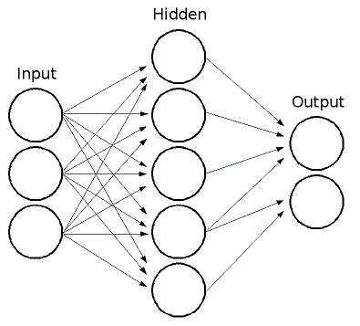
nn_model = MLPClassifier()
params = {'hidden_layer_sizes':[(100,), (150,)],'alpha':[0.0001, 0.01], 'activation':['tanh', 'relu'],
         'learning_rate':['adaptive','constant'], 'max_iter':[500]}
gs_nn = GridSearchCV(nn_model, params)
gs_nn.fit(X_train, Y_train)

gs_nn.best_params_

act = gs_nn.best_params_['activation']
alph = gs_nn.best_params_['alpha']
layer = gs_nn.best_params_['hidden_layer_sizes']
rate = gs_nn.best_params_['learning_rate']

nn_model = MLPClassifier(activation = act, alpha = alph, hidden_layer_sizes = layer,
                         learning_rate = rate, max_iter = 500)
nn_model.fit(X_train,Y_train)
print 'overall accuracy:', nn_model.score(X_test, Y_test)
prob_nn = nn_model.predict_proba(X_test)

pred_labels_nn = [0 if prob_nn[i][0] >.30 else 1 for i in range(len(prob_nn))]

cm_nn = confusion_matrix(Y_test, pred_labels_nn)
plot_confusion(cm_nn, classes, title = 'Neural Network Confusion Matrix')

tnr_nn = cm_nn[0,0]/float(cm_nn[0,0] + cm_nn[0,1])
print 'tnr:', tnr_nn

Majority Vote Ensemble
- Results from a set of models are combined to vote on the result.
mv_model = VotingClassifier([('xgb',xgb_model), ('nn', nn_model), ('lasso',best_lasso)], voting = 'soft')
mv_model.fit(X_train, Y_train)
print 'overall accuracy:', mv_model.score(X_test, Y_test)
prob_mv = mv_model.predict_proba(X_test)

pred_labels_mv = [0 if prob_mv[i][0] >.30 else 1 for i in range(len(prob_mv))]

cm_mv = confusion_matrix(Y_test, pred_labels_mv)
plot_confusion(cm_mv, classes, title = 'Majority Vote Confusion Matrix')

tnr_mv = cm_mv[0,0]/float(cm_mv[0,0] + cm_mv[0,1])
print 'tnr:', tnr_mv

Comparing Results
cmatrix = [cm_in, cm_lasso, cm_gb, cm_xgb, cm_nn, cm_mv]
models = ['Probation','Lasso','Gradient Boosting', 'XGBoost','Neural Network', 'Majority Vote']
classes = ['Not Returning', 'Returning']
tnr_values = [tnr_pj, tnr_lasso, tnr_gb, tnr_xgb, tnr_nn, tnr_mv]

def plot_all_confusion(cms, classes, titles):
    fig = plt.figure(figsize = (16,10))
    for i in range(1, len(cmatrix) + 1):
        j = i - 1
        cm = cms[j]
        ax1 = fig.add_subplot(2,3,i)
        sns.heatmap(cm, annot = True, fmt = 'd', annot_kws = {"size": 20}, ax = ax1,
                   xticklabels = ['Not Returning', 'Returning'],
                   yticklabels = ['Not Returning', 'Returning'],
                   cbar = 0,
                   cmap = "Blues")
        plt.xticks(rotation = 0, fontsize = 14)
        plt.yticks(rotation = 90, fontsize = 14)
        plt.title(titles[j] + ' tnr: ' + str(tnr_values[j]) , fontsize = 20)
        plt.tight_layout(h_pad = 5.0, w_pad = 3.0)
        plt.xlabel('Predicted Labels')
        plt.ylabel('True Labels')
plot_all_confusion(cmatrix, classes, models)

Remarks
This analysis was not done for consecutive semesters. Instead, I was interested in whether a student would return for a 3rd semester no matter how large the gap is between their 1st semester and 3rd semester. Even just looking into a few students who earned their degrees, several of them have taken a year to a year and a half off from school and return to finish their degree. This is not uncommon at a community college.
Improvements
More features outside of this dataset should give improvement to the results.
Knowing a students' age would help, especially for a community college because the range in age is greater than at a university. Many older adults return or enroll at community colleges.
Any geographic features regarding where students' reside would also improve results. From geographic data, more features can be engineered such as how far a student has to commute to school.
Job status would be an important feature. Having data on whether a student is working (part time vs full time) or is not working should drive improvements.
Finally, high school data such as standardized test scores, high school gpa, high school attended, and extracurricular activities participated in would defintely be important, especially when using the first semester data to predict retention.
Conclusion
- All of the machine learning models are an improvement compared to the current probation models
- The more appropriate model can be chosen depending on the amount of resources the school has
- The Neural Network provides the best true negative rate
- The more appropriate model can be chosen depending on the amount of resources the school has
- Application:
- Gain insights on students' risk status to intervene early, improving retention and persistence.
- Stronger basis on which students to allocate limited resources
- With a few modifications, this analysis can be used for any combination of semesters.